Practical 3: Models and their Structural Analysis
Once again, start ScrumPy as described previously.
Loading and defining models
A pre-existing model is loaded by creating an instance of a model object ScrumPy.Model(model) where model is a string type that is the name of the file containing the description of the model. If no name is provided, a pop-up file selector is launched. Conventionally, ScrumPy model files have the extension .spy, although this is not mandatory.
1 >>> m = ScrumPy.Model('toy_model.spy')
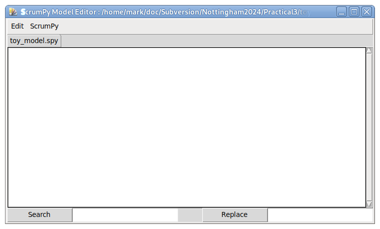
- If this file has not yet been created, the instruction will open a new empty editor window as shown:

Copy and paste the model description below. toy_model.spy is the small structural model described by:
Having done that, select "Compile" from the ScrumPy menu in the editor, and the model is saved loaded into ScrumPy. If you edit the model, you will need to Compile it again before the edits will be recognised.
The reactions with the suffix "_tx" are transporters, i.e. they convert external metabolites (with prefix "x_"), which can be consumed or produced, to internal metabolites, which have no net consumption or production at steady state. This is a convention, and a specific part of the model description language. Such conventions are invaluable when examining results generated from the analysis of large models
- Take a piece of paper and draw this reaction scheme as a metabolic pathway.
Having edited the model, before you can do any further analysis, you must tell ScrumPy to update the model internally by clicking the !ScrumPy/Compile menu option. This will also save the model, and as long as you have made no errors in entering it, you will see no further messages. You will be informed of any errors in a pop-up window, which will tell you where the error was first detected (not always the same as where the error is).
Properties of structural models
The class Model has a range of methods, of which some are only useful for kinetic models (which are also structural models, but the opposite is not true). The methods are actions on the model object (m in this case), and are invoked by instructions such as x = m.Method(), where the outcome is a new data object x that contains the result. Among the structurally relevant methods we find ConsMoieties() - which returns a list of conserved moieties; DeadReactions() - which returns a list of reactions that cannot carry steady state flux; FindIsoforms() - which identifies reactions from the model that are redundant, i.e. a set of reactions that have identical stoichiometry; ElModes() - which returns an elementary modes object; Externals() - which returns a list of external metabolites.
The stoichiometry matrix
The fields Model.sm and Model.smx are the two stoichiometry matrices associated with a model - the former is the internal matrix, the latter the external. The external matrix contains infomation about external metabolites, whereas the internal does not. All instances of ScrumPy matrices (subclasses of DynMatrix) have the fields cnames - column names and rnames - row names. Note that these are both lists, and can be examined as such.
Useful methods of sm (and smx) include ReacToStr(reac),
and InvolvedWith(name),
- Here, 'mpq(1,1)' is the stoichiometric coefficient for C, which for technical reasons is represented in the model object as an arbitrary precision rational number, i.e., 1/1 = 1, and as it is positive, C is a product. The coefficient for B is -1/1 = -1; it is a substrate of the reaction because its coefficient is negative.
Nullspace analysis
The kernel of the stoichiometry matrix can be calculated using the sm.NullSpace() method.
Even if the signs of some of the coefficients indicate thermodynamically infeasible solutions (e.g. all active reactions in the first column have negative coefficients, even though they are irreversible) a lot of useful information can be obtained form k. For instance, we see that the row associated with R_6 is a null-vector, indicating that there is no steady-state solution involving R_6. In fact this is how ScrumPy detects dead reactions with the method DeadReactions().
Enzyme subsets
Also, note that some of the row-vectors are proportional to each other - R_2, R_3; R_4, R_5; and E_tx, A_tx, R_1. This implies that these sets must carry flux in a coordinated fashion, e.g. any flux solution involving R_4 must also involve R_5. These sets of coordinated reactions are referred to as enzyme subsets and can be determined using the Model method EnzSubsets(). This method returns a dictionary object where keys are subset names (or reaction name if a reaction is in a singleton set) and values are nested dictionaries where keys are reaction names and values are the flux ratios of the reactions. The key DeadReacs maps to a list of dead reactions.
Elementary modes
The elementary modes of a model can be analysed using the method Model.ElModes(). This method returns an object that collects methods and fields related to the elementary modes of a given model. The member, .mo, is a matrix similar to k.
The relationship between modes and metabolites is stored in the sto matrix.
The methods Modes() and Stos() return strings with with same information as the matrices above.
Properties of the Stoichiometry Matrix and Null-space - Further Excercises
(a) Generate a kernel of the stoichiometry matrix (using the .NullSpace() method described above).
(b) Multiply the stoichiometry matrix by the kernel matrix, using the .Mul() method of the stoichiometry matrix.
(c) Repeat the multiplication above using the external stoichiometry matrix instead.
(d) Create a kernel of the external stoichiometry matrix - what is different?
(e) Multiply the internal and external stoichiometry matrices by your new kernel.
(f) Try adding or removing reactions from the model, and repeat the exercises above, explain the new results.