Kinetic Modelling
Contents
1. Loading a model
The general form of the description of a kinetic model has been covered in the pages on the ScrumPy Model Description Language. Consider this model file an example. It contains two reaction definitions with their kinetic equations, followed by initial assignments of the parameters and the variable (B). There are two limitations on the syntax for kinetic models:
- The identifiers cannot be quoted, and
- No C or C++ key words can be used as identifiers.
pH = 7.5
k2eq = 17.84e8*10**(-pH)
If the two reaction model above is saved as a spy file, it can be loaded into ScrumPy to create an instance of a model object as follows:
m = ScrumPy.Model()
See Loading a model for more details.
2. Inspecting and assigning values
- Once it has been loaded, values can be inspected, e.g.:
>>> m[ " x_A " ]    # parameter
1 . 0
>>> m[ "B" ]        # concentration
0.4
>>> m[ "R1" ]       # rate, evaluated with current variable values
3.3333333333333335
>>> m[ " x_A " ] = 2   # parameter
>>> m[ "B" ] = 2       # concentration
>>> m["R1"]
3.3333333333333335
>>> m.Eval()
>>> m["R1"]
2.0
That is, the computation of the rate is not updated until m.Eval() is called to force a re-evaluation of the rate with current parameters and concentration values.
The following table shows the methods/attributes of any model instance m that return lists of the corresponding entities:
Constituent
Values
Identifiers
Parameters
m.GetVec(ScrumPy.Param)
m.ParamNames
Metabolites
m.GetVec(ScrumPy.Conc)
m.sm.rnames
Metabolite rates of change
m.GetVec(ScrumPy.dMet)
m.sm.rnames
Reaction rates
m.GetVec(ScrumPy.Vel)
m.sm.cnames
The corresponding method SetVec takes as parameters one of the same codes as GetVec followed by a vector of values, but the vector must be the correct length ( as indicated by, e.g. len(m.ParamNames)).
2.1. Moiety conservation parameters
ScrumPy takes care of any dependencies between metabolites by computing the moiety conservation relationships from the stoichiometry matrix. These arise, for example, where coenzymes such as NAD and NADH occur in a model, but the nucleotide moieties are not synthesised and degraded by the model reactions.
In such cases, a new parameter, with an identifier starting CSUM_, is created and assigned a value that is the sum of the initialised concentrations of the metabolites in the conservation group. One of the metabolite concentrations will then not be integrated, but will have its concentration determined as the difference between the CSUM parameter and the sum of all the remaining metabolite concentrations.
It is strongly recommended that you do not try to anticipate dependencies by manually eliminating one of the conserved group metabolites from your model. ScrumPy uses a mathematically-validated method to determine the conservation relationships, which can be complicated and non-intuitive, especially where two conservation groups intersect. Furthermore, without the conservation sum constraint, steady state solvers cannot be guaranteed to respect the conserved total.
As an example, if the model SimpleCycle.spy is downloaded, saved and load into ScrumPy, the following commands can be issued:
>>> m.ParamNames
['x_A', 'x_C', 'CSUM_NADH']
>>> m.GetVec(ScrumPy.Param)
[2.0, 1.0, 1.0]
>>> m.ConsMoieties()
    NAD

 NAD 1/1
 B 0/1
 C 0/1
 NADH 1/1
>>> m.ConsDic()
{'NAD': [('NADH', mpq(1,1))]}
m.ParamNames shows that an additional papameter, CSUM_NADH has been created, and m.GetVec(ScrumPy.Param) shows this has been initialised as 1. m.ConsMoieties() returns a single vector showing there is one conservation relationship, involving 1 NAD and 1 NADH. (1/1 is the rational fraction representation of 1). m.ConsDic() conveys the same information, but returns the dependency as a dictionary, with mpq(1,1) being another representation of the rational fraction 1/1.
3. Examining steady states of the model
The steady state of the model can be determined with m.FindSS(); if the steady state is found successfully, than m.IsOK() will return True.
A straightforward way to record a series of steady states as a parameter is changed uses the AddStatMonitor method from the DataSets class, described in more detail elsewhere. For example:
>>> results=m.AddStatMonitor()
>>> m["x_A"]=1
>>> m.FindSS()
>>> for n in range(20):
        m["Vmax1"] += 1
        m.FindSS()
        print m.IsOK()
results is a ScrumPy matrix, the columns of which (results.cnames) contain the time, rates, concentrations and parameter values of the model (though the time is always zero in this case). A row is added to the matrix with each successful steady state determination, recording the steady state values.
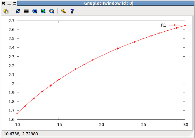
There are methods for plotting the outcome of the set of analyses that are described more fully in Secondary Analysis of Model Results (link to be made). A simple example is:
>>> results.SetPlotX("Vmax1")
>>> results.AddToPlot("R1")

3.1. What to do if a steady state is not found
Before looking for potential problems with the numerical solution of your model, check via structural analysis (insert links) that your model has elementary modes connecting inputs to outputs, and that there are no structurally dead reactions (other than those that can attain equilibrium).
The FindSS method may not converge if the initial estimates of the variables are not close enough to the steady-state values. One way to move the variables closer to their steady state values is by a time course simulation. In fact, the FindSS method will automatically try this if it initially fails to find a steady state. However, the simulation time it uses is relatively short. Hence it might be worth explicitly running a time course simulation (see LINK) to see whether the model is or is not appearing to tend to a stable steady state.